Abstract

It is well-understood that properly designed lighting is critical for implementing a robust, and timely vision inspection system. A basic understanding of illumination types and techniques, geometry, filtering, sensor characteristics, and color, as well as a thorough analysis of the inspection environment, including part presentation and object-light interactions, provide a solid foundation when designing an effective vision lighting solution. Developing a rigorous lighting analysis will provide a consistent, and robust solution framework, thereby maximizing the use of time, effort, and resources.

Introduction

Perhaps no other aspect of vision system design and implementation has consistently caused more delay, cost-overruns, and general consternation than lighting. Historically, lighting was often the last aspect specified, developed, and or funded, if at all. And this approach was not entirely unwarranted, as until recently there was no real, vision-specific lighting on the market; lighting devices were often consumer-level incandescent or fluorescent lighting products.

The objective of this paper, rather than to dwell on theoretical treatments, is to present a “Standard Method for Developing Feature Appropriate Lighting”. We will accomplish this goal by detailing relevant aspects, in a practical framework, with examples, where applicable, from the following three areas:

1. Familiarity with the following four Image Contrast Enhancement Concepts of vision illumination:
   • Geometry
   • Pattern, or Structure
   • Wavelength
   • Filters
2. Detailed analysis of:
   • Immediate Inspection Environment – Physical constraints and requirements
   • Object – Light Interactions with respect to your unique parts, including ambient light
3. Knowledge of:
   • Lighting types, and application advantages and disadvantages
   • Vision camera and sensor quantum efficiency and spectral range
   • Illumination Techniques and their application fields relative to surface flatness and surface reflectivity
   • When we accumulate and analyze information from these three areas, with respect to the specific part/feature and inspection requirements, we can achieve the primary goal of machine vision lighting analysis — to provide object or feature appropriate lighting that meets two Acceptance Criteria consistently:
     1. Maximize the contrast on those features of interest vs. their background
     2. Provide for a measure of robustness

As we are all aware, each inspection is different, thus it is possible, for example, for lighting solutions that meet Acceptance Criterion 1 only to be effective, provided there are no inconsistencies in part size, shape, orientation, placement, or environmental variables, such as ambient light contribution (Fig. 1).

Review of Light for Vision

For purposes of this discussion, light may be defined as photons propagating as an oscillating transverse electromagnetic energy wave, characterized by both magnetic and electric fields, vibrating at right angles to each other – and to the direction of wavefront propagation – (Fig. 2).

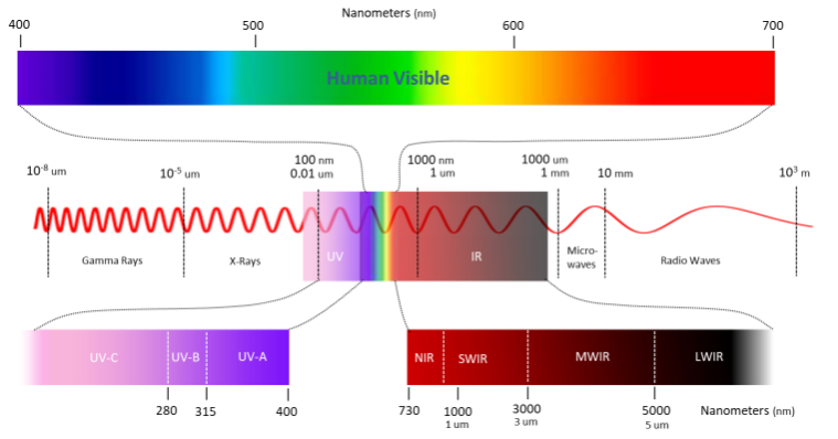
The electromagnetic spectrum encompasses a wide range of wavelengths, from Gamma Rays on the short end, to Radio Waves on the long end, with the UV, Visible, and IR range in the middle. For purposes of this discussion, we will concentrate on the Near UV, Visible and Near IR regions (Fig. 3).

Light may be characterized and measured in several ways:

1. Measured “Intensity”:
   • Radiometric: Unweighted measures of optical radiation power, irrespective of wavelength in Watts (W) per unit area
   • Photometric: Perceived light power of radiometric measures – weighted to the human visual spectral response and confined to the “human visible” wavelengths in lux (lx = lumens / m²)
2. Frequency: Hz (waves/sec)
3. Wavelength: Expressed in nanometers (nm) or microns (um)

In machine vision applications, we tend to express light in wavelength units (nm) preferentially over frequency; therefore, we will stress the following relationships among light wavelength, frequency, and photon energy with respect to wavelength. All three of these properties are also related to the speed of light as expressed by the following two equations:

1. c = λƒ
2. c = λE / h (Planck’s Equation), where:

c = speed of light

E = photon energy

λ = wavelength

h = Planck’s constant

ƒ = frequency expressed in Hz

Combining the two formulas by canceling c and solving for E, we arrive at the relationship known as the Planck – Einstein equation:

E = hƒ

From these manipulations we see there are two important relationships that we can use to our advantage when applying different wavelengths to solving lighting applications:

1. wavelength and frequency are inversely proportional ( λ ~ 1 / ƒ )
2. wavelength and photon energy are inversely proportional ( λ ~ 1 / E )

From a practical application standpoint, we can best apply these two relationships to assist in creating feature-specific image contrast, particularly when we analyze how light of different wavelengths interacts with surfaces.

Additionally, it is important to note that the human visual system and CCD/CMOS or film-based cameras differ widely in two important respects: Photon sensitivity and wavelength range detection (See Figs. 4, 5).

Vision Illumination Sources

The following lighting sources are now used in machine vision:

• Fluorescent
• Quartz Halogen – Fiber Optics
• LED – Light Emitting Diode
• Metal Halide (Mercury)
• Xenon (Strobe)

LED, fluorescent, quartz-halogen and Xenon (Figs. 6a-j) are by far the most widely used lighting types in machine vision, particularly for small to medium-scale inspection stations, whereas metal halide and Xenon are more often deployed in large-scale applications, or applications requiring a very bright source. Metal halide, also known as mercury, is often used in microscopy because it offers many discrete wavelength peaks, which complements the use of filters for fluorescence studies.

A Xenon source is useful for applications requiring a very bright, strobe light. Fig. 7 shows the advantages and disadvantages of Xenon, fluorescent, quartz halogen, and LED lighting sources, in accordance with relevant selection criteria, as applied to machine vision. For example, whereas LED lighting has a longer life expectancy, fluorescent lighting may be the most appropriate choice for a large-area inspection because of its lower cost per unit illumination area – depending on the relative merits of each to the application.

Historically, fluorescent and quartz halogen lighting sources were most often used for machine vision applications. However, over the last 15 years, LED technology has consistently improved in stability, intensity, efficiency, and cost-effectiveness to the extent that is now accepted as the de facto standard for almost all mainstream applications. On the other hand, fiber-coupled quartz halogen sources are still a go-to solution for many microscopy/lab applications. While LED sources are not yet providing the same levels of intensity and output/price performance of Xenon strobe sources, high-speed image capture is still possible with LED-based strobe lighting, as evidenced by the images in Fig. 8, showing a bullet breaking light bulbs and cutting a playing card.

It should also be noted at this time that many of the examples and results demonstrated and described in this document were generated using LED sources, unless otherwise indicated, rather than the other aforementioned source types; however, many of these results could also be adequately replicated with other sources.

Understanding Radiometric and Photometric Measurement

As elaborated earlier, light “intensity” is expressed Radiometrically or Photometrically. The Machine Vision Industry has often followed the commercial lighting practices of specifying light source-only power in Watts (radiometric) or lumens (photometric), whether it is white light or other monochromatic sources (red, green, blue,). The primary two pitfalls when evaluating lights based on specifications are:

1. Source power only: No information with respect to “the amount of light” cast on an object.
2. Comparing – on paper -white light intensity vs. that of monochromatic light in photometric, rather than radiometric values.

From a practical viewpoint, a MV Engineer or Technician benefits the most, conceptually, when they can compare light intensities on an object in the real world, primarily at a known light working distance (WD) for front lighting and at an emitting surface for back lighting – this opposed to simple source-only power specification.

The power specification of a lighting source (in W or lm), by definition, offers neither information about the light intensity at a distance nor light travel geometry – is it a spherical source, like the Sun, radiating light in a spherical front, or focused in a direction, like a flashlight? As we all know, how light is or is not focused from a source plays a major role in the intensity available on the surface of an object we might be inspecting – even if the source-only intensities are otherwise identical.

It is advantageous, therefore, to consider light intensity specification that takes light travel geometry into account as Irradiance (W/m2) or Illuminance in Lux (lx – lm/m2) as a measure of radiant power. For these reasons we will use the more machine vision appropriate term, “radiant power” when referring to the “amount of light on a surface”.

(Please see Appendix B – Extended Topic 1 – for a more technically detailed examination of lighting ‘intensity” involving both source and light travel geometry concepts).

The key cause of confusion when understanding and applying radiometric vs. photometric radiant power specification, especially when comparing white against monochromatic sources or among the latter is related to the simple fact that photometric source output is weighted to the human eye response to color, as we saw from Fig. 4. For example, this means that because humans do not see IR or UV light, a photometric specification lists their intensities as “0” – not practical for comparison purposes.

Consider the following comparison of radiometric vs. photometric light “intensity” in the table depicted in Fig 9:

Clearly, whereas this information is not incorrect, it’s just easily misinterpreted without proper context and understanding.

We can see a real-world example of how easy it is to be misled when selecting a “most-appropriate” wavelength for an application. Consider that a vision tech has been tasked with selecting an LED wavelength with the “brightest” output because the application is suspected of being light-starved. For example, the application could require very short exposure times in order to freeze motion due to high object speeds, which of course forces an increase in light intensity to compensate for the shorter light collection time.

The vision tech then locates the following graphic (Fig. 10) of LEDs, based on a photometric (human vision weighted) specification. It’s very easy to select the green 565 nm LED based on the listed relative intensities.

However, if we take note of the same LED intensities, but specified in radiometric (unweighted) terms, we potentially have quite a different selection outcome (Fig. 11). Clearly, from the standpoint of un-weighted radiant power output, the IR LEDs might be the obvious choice, but we must consider a camera sensor’s Quantum Efficiency (QE) curve: This is illustrated by the green line – the camera is not particularly IR sensitive, therefore, it is not a viable solution.

Additionally, the other relevant information from the data portrayed in Fig. 11 is the stark difference in actual radiant power of the shorter wavelengths (green 525nm and blue 470nm) specified radiometrically vs. photometrically. The camera is also the most sensitive to the blue 470 (with peak sensitivity a bit above that). Therefore, the obvious choice to offer the most radiant power that is also the most efficiently collected is the blue 470nm light.

For these reasons, there are a few rules-of-thumb to consider when comparing specified intensities:

1. Compare monochromatic vs. all wavelengths, including white light, by irradiance (radiometric).
2. Compare white vs. white light intensity by illuminance or irradiance.
3. Compare intensities in the same units and measured at the same WD.
4. Consider your camera sensor’s QE when making wavelength selections.

The Table in Fig. 12 graphically summarizes the above information.

The Light Emitting Diode

A light emitting diode (LED) may be defined as a semiconductor-based device that converts electrons to light photons when a current is applied. The emitted wavelength (referred to as color in the visible range) is determined by the energy required to allow electrons to jump the materials’ valence to conduction band gap, thus producing wavelength-specific photons. The efficiency of this electron to photon conversion process is reported as source lumen efficacy, and is often expressed as lm/W.

An important concept for specifying monochromatic LED performance, particularly in scientific disciplines is spectral full-width, half-max (FWHM). Basically, this is a measure of the spectral curve width, specified at the 50% intensity point after subtracting the noise floor values from the total spectral curve height (please see Appendix B – Extended Topic 2 for a more detailed discussion about spectral and image intensity FWHM).

Available LED wavelengths, radiant power and lumen efficacy have increased rapidly in the last 20 years, including white LED development spurred on by the commercial lighting industry. It should be noted that there are no LED die that directly generate a visible white spectrum, but rather blue LEDs provide the excitation wavelength to create a secondary emission (fluorescence) of yellow phosphors under the LED lens. For this reason, the commercial introduction of “white” LEDs had to await the perfection of blue LED technology in the mid-1990s. For more background, see:

https://en.wikipedia.org/wiki/Light-emitting_diode)

https://www.vision-systems.com/cameras-accessories/article/14232797/leds-the-swiss-army-knives-of-machine-vision-illumination

Similarly, LED design has evolved of the years, particularly with respect to thermal management. Although LEDs are very efficient generators of light, they are not 100% efficient and hence as the radiant power has increased, so has the need for localized LED thermal management (see Fig. 13).

It is important to consider not only a source’s brightness, but also its spectral content (Fig. 14). Fluorescence microscopy applications, for example, often use a full spectrum metal-halide (mercury) source, particularly when imaging in color; however, specific wavelength monochromatic LED sources are also useful for narrow-wavelength output biomedical requirements using either a color or B&W camera.

In those applications requiring high light intensity, such as high-speed inspections, it may be useful to match the source’s spectral output with the spectral sensitivity of the proposed vision camera (Fig. 15) used.  For example, CMOS sensor-based cameras are more IR sensitive than their CCD counterparts, imparting a significant sensitivity advantage in light-starved inspection settings when using IR LED or IR-rich Tungsten sources.

Additionally, the information in Figs. 14-15 illustrates several other relevant points to consider when selecting a camera and light source.

• Attempt to match your camera sensor’s peak spectral efficiency with your lighting source’s peak wavelength to take the fullest advantage of its output, especially when in light-starved high part speed applications.
• Narrow wavelength sources, such as monochromatic LEDs, or mercury are beneficial for passing strategic wavelengths when matched with pass filters. For example, a red 660nm band pass filter, when matched to a red 660nm LED light, is very effective at blocking ambient light on the plant floor from overhead fluorescent or mercury sources.
• Ambient sunlight has the raw intensity and broadband spectral content to call into question any vision inspection result – use an opaque housing.
• Even though our minds are very good at interpreting what our eyes see, the human visual system is woefully inadequate in terms of ultimate spectral sensitivity and dynamic range – let your eyes view the image as acquired with the vision camera.

LED Lifetime Specification

As is clear from the discussion and graphic presented earlier, LEDs offer considerable advantages related to output and performance stability over their significant and useful lifetimes. When LEDs were still manufactured primarily as small indicators, rather than for effective machine vision illuminators, the LED manufacturers specified LED lifetime in half-life; as the industry matured and the high-brightness LEDs became commonplace for commercial and residential application, manufactures were pushed to specify a more practical and understandable measure of performance over their lifetimes, referred to as “lumen maintenance”. Please see Appendix B – Extended Topic 3 for a more detailed examination.

White LED Correlated Color Temperature

We are now familiar with commercial and residential white LED lights, where illuminator color temperature (expressed in degrees Kelvin – K) may be understood as the relative amount of red vs. blue hue in the light content. This can vary from warm 2000K – 4000K, neutral 4000K – 5500K, and cool 5500K – 8000K plus. With respect to machine vision applications, the amount of blue or red content in a white LED illuminator can have a significant effect on the inspection result, depending on the application, particularly on color applications. Color inspections may require accurate image color representation for the purposes of reproduction, identification, object matching/selection or quality control of registered colors. To be successful, it is necessary to understand two light measurement parameters: white light LED correlated color temperature (CCT) and color rendering index (CRI).

For a more detailed examination of white light color temperature application in machine vision, please see Appendix B – Extended Topic 4.

Photobiological Safety Considerations

As LEDs have become more powerful – and more prevalent on the manufacturing floor, occasionally placing them near human operators, eye safety has become a priority, particularly in strobing operations. Initially, LEDs were classified under the laser safety categories by class. However recently the International Electrotechnical Commission (IEC) has reclassified LED light into its own set of categories, collectively known as, and detailed by, an IEC 62471 document. The commission subdivided the Near UV to Near IR wavelength ranges, including visible, into five definable hazard types (see left side vertical column of Fig. 16). A light “luminaire” is typically tested against a set of well-documented standards and is then assigned into 1 of 4 Risk Groups, ranging from “Exempt” Risk through High Risk (Groups 0-3, respectively). Additionally, a companion document IEC 62471-1 offers Guidance Control Measures for mitigation – See Fig. 16. All machine vision lighting vendors now offer light Safety Risk Group designations for their lights.

There is some overlap in the Hazard areas, because of the mix of possible wavelength ranges for some lights. Further, it’s important to note the differences between dermal and eye contact hazards for IR. Upon contact to dermal areas, IR light is simply absorbed by the skin and therefore does not pose a hazard under normal exposure conditions. Whereas, upon penetration of the eye, IR light produces no eye response, and unlike a visible light reaction, the eye neither closes down the iris, nor produces an eye aversion response that generally protects the retina from damage as it does with visible light. If the IR light is sufficiently strong, it can produce heat as it’s absorbed into the back of the eyeball – and that can cause damage to the retina and perhaps the optic nerve. As of this writing, most of the near and short-wavelength IR lights used in machine vision do not offer the radiant power to induce retinal damage and are therefore classified as either Exempt Risk or Risk Group 1. Always consult the lighting manufacturer if any question as to their safety.

The Standard Method in Machine Vision Lighting

In the Introduction, we listed three relevant aspects necessary to develop a Standardized Lighting Method. They are:

1. The four Image Contrast Enhancement Concepts (Cornerstones)
2. Detailed inspection environment and light-object Interaction Analysis, including ambient light contributions
3. Knowledge of Lighting Techniques/Types, and camera sensor QE

These, along with the accumulated application, discovery process and testing results, when considered together, can lead to a lighting solution that produces feature-appropriate contrast consistently and robustly.

The Four Cornerstones of Image Contrast

These concepts were devised as a teaching tool for labelling and demonstrating four methods applied to enhance or even create feature–appropriate image contrast of parts vs. their backgrounds. The goal is to have effective, consistent, and robust features defined as best suited for a given inspection.

The four Image Contrast Enhancement Concepts of vision illumination are:

1. Geometry – The spatial relationship among object, light, and camera:
   
2. Structure, or Pattern – The shape of the light projected onto the object:
   
3. Wavelength, or Color – How the light is differentially reflected or absorbed by the object and its immediate background:
   
4. Filters – Differentially blocking and passing wavelengths and/or light directions:
   

A common question raised about the four Image Contrast Enhancement Concepts is priority of investigation. For example, is wavelength more important than geometry, and when to apply filtering? There is no easy answer to this question, and of course the priority of investigation is highly dependent on the part and the expected application-specific results. Light Geometry and Structure are more important when dealing with specular surfaces, whereas wavelength and filtering are more crucial for color and transparency applications.

Understanding how manipulating and enhancing the image contrast from a part, or part feature of interest, against its immediate background, using the four Concepts is crucial for assessing the quality and robustness of the lighting system. It should be noted that it is not at all uncommon to utilize more than one Concept to solve an application, and in some cases they may all need to be used. In fact, the following description and examples from each Concept category show considerable overlap for just this reason.

Cornerstones 1 & 2 Geometry: Pattern and Structure

Although the term, Geometry, is used generically, it is sometimes useful to differentiate System Geometry vs. Light Ray Geometry. System Geometry is defined as that spatial relationship among the camera, light head and part or feature of interest – see Fig. 17. In general, there are two broadly defined System Geometries – Coaxial Lighting (on-axis) and Off-axis Front Lighting – we can consider back lighting as a coaxial variant as well. Coaxial implies the light is centered about the camera’s optic axis, but there is no definition or expectation of how the camera is positioned with respect to the part surface.

Effecting contrast changes via Geometry involves moving the relative positions among object, light, and/or camera in space until a suitable configuration is found. This combination of moves in space is most amenable under partial brightfield, directional lighting (see later section – “Partial Bright Field Lighting”), however. Full brightfield, diffuse techniques tend to require fixed and coaxial alignment positions between the light and camera/lens, thus restricting the full degree of relative component movement.

Light Ray Geometry may be related to System Geometry – in the sense that certain System Geometries produce specific Light Ray Geometries, however, sometimes the same off-axis System Geometry may produce a different effect on the part or features of interest, particularly in the case of reflection geometry – as seen in Fig. 18. Specifically, the light and resulting image produced in a Coaxial System Geometry (camera and light), in an Off-axis orientation (Fig. 18a) will be considerably different from both the camera and light in off-axis, non-coaxial positions (Fig. 18b).

The Light Ray Geometry illustrated in the left graphic in Fig. 18 is designed to mitigate surface specular reflection so relevant surface details are visible in an image, whereas that depicted in the right graphic is designed to gather, rather than mitigate reflections – usually because the features of interest are differentially more reflective in contrast to the rest of the surface.

As can be surmised, the type of inspection under the System and Light Ray Geometries depicted in Fig. 18 is generally limited to Presence/Absence or perhaps general location, rather than any measurement for sizes, shapes, or spatial relationships, owing to the off-axis perspective of the camera with respect to the surface. In this instance, we can alleviate surface glare by keeping the camera perpendicular to the inspection surface and moving the light off-axis to some degree (Fig. 19), thus accomplishing the same surface glare mitigation without the perspective shift in the image.

Contrast changes via Structure, or the shape of the light projected on the part is generally light head, or lighting technique specific (See later section on Illumination Techniques). Contrast changes via Color lighting are related to differential color absorbance vs. reflectance (See Object – Light Interaction).

Figure 20 illustrates another example how crucial Geometry is for a consistent and robust inspection application on a specular cylinder.

The application of some techniques requires a specific light and geometry, or relative placement of the camera, object, and light; others do not. For example, a standard bright field bar light may also be used in a dark field orientation, whereas a diffuse dome light is used exclusively in a coaxial mount orientation.

Most manufacturers of vision lighting products offer lights that can produce various combinations of lighting effects, and in the case of LED-based products, each of the effects may be individually addressable. This allows for greater flexibility and reduces potential costs when numerous inspections can be accomplished in a single station, rather than two. If the application conditions and limitations of each of these lighting techniques, as well as the intricacies of the inspection environment and object–light interactions are well understood, it is possible to develop an effective lighting solution that meets the two Acceptance Criteria listed earlier.

Illumination Techniques

Illumination techniques comprise the following:

• Back Lighting
• Diffuse Lighting (also known as full bright field)
• Bright Field (partial or directional)
• Dark Field
• Structured Lighting

Back Lighting

Back lighting generates instant image contrast by creating dark silhouettes against a bright background (Fig. 21). The most common uses are detecting presence/absence of holes and gaps, part placement or orientation, or gauging. It is often useful to use a monochrome light, such as red, green, or blue, with collimation film for more precise (subpixel) edge detection and high accuracy gauging. Back lighting is also beneficial for transmitting through transparent or semi-transparent parts, such as the glass bottle imaged in Fig. 21b using a red 660 nm light source.

A variant of the backlight is designed specifically for line scanning applications deploying a high-speed linescan camera, typically on fast moving webs (see more detail in a subsequent section on linescan lighting). These linear backlights have a long, narrow form-factor and are designed to produce the extreme intensities that are necessary to handle the camera’s high line rates, needed to freeze motion. These applications and are most often deployed to penetrate and inspect thin web materials. A good example is perforation detection in plastic bag stock before forming into bags, or dislocations in the weave of a semi-transparent textile web. Constant-on, rather than strobing is the rule in these cases.

Partial Bright Field Lighting

Partial (directional – see Fig. 22) bright field lighting is the most commonly used vision lighting technique, and is the most familiar lighting we use every day, including sunlight, lamps, flashlights, etc. It is typically produced by spot, ring, or bar light style lights. This type of lighting is distinguished from full bright field in that it is directional, typically from a point source, and because of its directional nature, it is a good choice for generating contrast and enhancing topographic detail. It is much less effective, however when used on-axis with specular surfaces, generating the familiar “hotspot” reflection (Fig. 22).

Full Bright Field Lighting

Diffuse, or full bright field lighting is commonly used on shiny specular, or mixed reflectivity parts where even, but multi-directional/multi-angle light is needed. There are several implementations of diffuse lighting generally available, but three primary types, hemispherical dome/tunnel or on-axis (Figs. 23a-c) being the most common.

Diffuse dome lights are very effective at lighting curved, specular surfaces, commonly found in the automotive industry, for example. Diffuse dome lights are most effective because they project light from multiple directions (360 degrees looking down the optic axis) as well as multiple angles (from low to high), which tends to normalize differential surface reflections on complex shape parts.

On-axis (Coaxial) lights work in similar fashion as diffuse dome/tunnel lights for flat objects, and are particularly effective at enhancing differentially angled, textured, or topographic features on otherwise planar objects. A useful property of Coaxial diffuse lighting is that in this case, rather than mitigating or avoiding specular reflection from the source, we may rather take advantage of the it – if it can be isolated specifically to uniquely define the feature(s) of interest required for a consistent and robust inspection (see Fig. 24).

Flat diffuse lighting may be considered a hybrid of dome and Coaxial diffuse lighting. From a lighting geometry standpoint, it produces more off-axis light rays than a coaxial light, but fewer than a dome light. Because the flat diffuse light is direct lighting, rather than internally reflected from within a dome light to the object, this light can be deployed over a much wider range of light working distances, especially longer WD not possible with a dome light.

In the image sequence in Fig. 26a, we see a titration tray of wells – approximately 4” x 5” in size. The base of each 5mm wide and tall well has a laser-etched 2-D code, where the contents of each well is stored and identified by the data contained in each 2-D code. The inspection goal was to read the codes in each well base. Clearly, a higher magnification was necessary to resolve the small code details, and a 2×3 size code area was utilized to unambiguously illustrate the well’s response to different lighting geometries.

High angle, direct lighting (Figs. 26b-c) clearly produces unacceptable results in not meeting acceptable feature-specific part/background contrast, in this case, the codes against their immediate background. Low angle light (Fig. 26d) improves the code contrast which may well be an acceptable solution. However, looking more closely at the upper right well, we do notice a crescent shaped shadow. This is to be expected if we consider that the wells do have walls that are not otherwise conspicuous in this largely top-down lighting geometry sequence. The crescent is formed because the walls are vignetting the light somewhat, but not to the extent to otherwise block the view of the 2-D code. Nonetheless, we do have to consider whether this low angle ring light solution is robust enough to be effective for all part presentation situations and circumstances. For example, had the codes been offset sufficiently from the center, they may have been vignetted, precluding adequate reading.

The diffuse dome light, as advertised, delivers a very even contrast image, but does not actually highlight the codes against their backgrounds (Fig. 26e), and we can see, the flat diffuse dome lighting offers the most effective and robust solution (Fig. 26f), and unlike the diffuse dome, its geometry does not require mounting the light very close to the parts. Clearly, this example demonstrates why it’s often important to test a wide variety of geometries. The author was convinced before testing that the diffuse dome was the best solution, which turned out to not be the case!

Dark Field Lighting

Dark field lighting (Fig. 27) is perhaps the least well understood of all the techniques, although we do use these techniques in everyday life. For example, the use of automobile headlights relies on light incident at low angles on the road surface, reflecting from the small surface imperfections, and other objects.

Dark field lighting can be subdivided into circular and linear (directional) types, the former requiring a specific light head geometry design. This type of lighting is characterized by low or medium angle of light incidence, typically requiring a very short light working distance, particularly for the circular light head types (Fig. 28b).

Bright Field vs. Dark Field

The following figures illustrate the differences in implementation and result of circular directional (partial bright field) and circular dark field lights, on a mirrored surface:

Effective application of dark field lighting relies on the fact that much of the low angle (<45 degrees) light incident on a mirrored surface that would otherwise flood the scene as a hot-spot of glare, is reflected away from, rather than toward the camera.

The relatively small amount of light scattered back into the camera happens to catch an edge of a small feature on the surface, satisfying the “angle of reflection equals the angle of incidence” equation (See Fig. 29 for another example).

The seemingly complex light geometry distinctions between bright and dark field lighting can best be explained in terms of the classic, “W” concept (Fig. 30).

To complicate matters, the standard, symmetric “W” pattern illustrating classic dark vs. bright field lighting can be considerably distorted as well. In the above illustration, the camera is mounted such that its optic axis is perpendicular to the surface being imaged, which is of course typical to minimize surface image perspective shifts.

However, imagine if the camera and integrated light (built into the face of the camera), or attached ring light, were mounted such that their optic axes were no longer perpendicular to a surface being imaged, but also not off-axis by 45 degrees or more (normally understood to be dark-field light angle of incidence), what would we expect to see in the resulting image?

Another important aspect of dark field lighting is its flexibility. Many standard partial bright field lights can be used in a dark field configuration. This technique is also very good for detecting edges in topographic objects, and the directional variety can be used effectively if there is a known, standard or structured feature orientation in an object, not otherwise requiring 360 degrees of light direction to generate contrast. A good example of this is a scratch generated on continuous sheet steel caused by something on the conveyor belt, creating a continuous longitudinal scratch. In this instance, a low angle directional light pointing across the web/conveyor will highlight the scratch very easily and consistently.

Structured Line Lighting

A much more thorough explanation of line lighting and linescan cameras is available here from Vision Systems Design:

https://www.vision-systems.com/cameras-accessories/article/14215087/lighting-for-line-scan-imaging

Not all linescan applications require hi-power output, however. A common early application that required relatively low intensity was the imaging of can labels. The can was typically rotated and imaged around the long axis under the light and linescan camera, creating a large, “unwrapped” 2-D image.

Application Fields

Figure 33 illustrates potential application fields for the different lighting techniques, based on the two most prevalent gross surface characteristics:

1. Surface Flatness and Texture
2. Surface Reflectivity

This diagram plots surface reflectivity, divided into three categories, matte, mirror, and mixed versus surface flatness and texture, or topography. As one moves right and downward on the diagram, more specialized lighting Geometries and Structured Lighting types are necessary.

As might be expected, the “Geometry Independent” section implies that relatively flat and diffuse surfaces do not necessarily require specific lighting, but rather any light technique may be effective, provided it meets all the other criteria necessary, such as working distance, access, brightness, and projected pattern, for example – and produces the necessary feature-appropriate image contrast needed for the inspection.

Cornerstone 3: Color / Wavelength

Materials reflect and/or absorb various wavelengths of light differentially, an effect that is valid for both B&W and color imaging space. It is important to remember that we perceive an object as red, for example, because it preferentially reflects those wavelengths our minds interpret/perceive as red – the other colors in white light are absorbed, to a greater or lesser extent. As we all remember from grammar school, like colors reflect, and surfaces are brightened; conversely, opposing colors absorb, and surfaces are darkened.

Using a simple color wheel of Warm vs. Cool colors (Fig. 34), we can generate differential image contrast between a part and its background (Fig. 35), and even differentiate color parts, given a limited, known palette of colors, with a B&W camera (Fig. 36). Opposite colors on the wheel generate the most contrast differences, i.e. – green light suppresses red reflection more than blue or violet would. And this effect can be realized using actual red vs. green vs. blue colored light (sometimes referred to as narrow-band light), or via filters and a white light source (broad-band source). What is critical to remember is we are evaluating how a part or feature responds to incident light of a specific color – with respect to its background color and/or reflectivity profile. This point also begs the question: what about IR light for creating contrast? More on this in a later section.

Object Properties – Absorption, Reflection, Transmission and Emission

Object composition can greatly affect how light interacts with objects. Some plastics may only transmit light of certain wavelength ranges, and are otherwise opaque; some may not transmit, but rather internally diffuse the light; and some may absorb the light only to re-emit it at a different wavelength (fluorescence).

From an earlier discussion we know that fluorescence is a secondary process by which a specific excitation source (most often, but not necessarily confined to UV wavelengths) illuminates a material that emits a longer wavelength. UV based fluorescence labels and dyes are commonly “doped” into inks for the printing and security industries (see Figs. 37a-b). This technique is invaluable for disguising information a manufacturer does not want the consumer to see. It is often used in the security field, particularly to thwart counterfeit money or passports and other official items and materials. Some materials naturally fluoresce under UV light, such as nylon structural fibers in cloth material – in this case the fluorescent emission wavelength is blue (Fig. 37c).

One obstacle to overcome when deploying UV fluorescence, concerns the emission light’s overall intensity. Secondary emissions consist of lower energy photons, so the relatively weaker fluorescent yield can be easily contaminated and overwhelmed by the overall scene intensity, particularly when ambient light is involved. In addition to blocking ambient “noise” to prefer the projected visible light with which we illuminate an object, band-pass filters on the camera lens also provide critical ambient blocking function in fluorescence applications, but with added functionality: The filter can be selected to prefer the emission wavelength, rather than the source light wavelength projected on the part – and in fact it performs the dual function of blocking both the UV source and ambient contributions that combine to dilute the emission light signal (Fig. 38). This approach is effective because once the UV light has fluoresced the part or features of interest, it is then considered ambient noise.

The properties of IR light can be useful in vision inspection for a variety of reasons. First, IR light is effective at neutralizing contrast differences based on color, primarily because reflection of IR light is based more on object composition and/or texture, rather than visible color differences. This property can be used when less contrast, normally based on color reflectance from white light, is the desired effect (See Fig. 39).

Unlike the image results depicted in Fig. 39, where the NIR light actually changes the reproduced content of the image, the following example diminishes color contrast differences on a line-up of crayons (Fig. 40) – while simultaneously increasing contrast of the hard-to-read print crayon. The black print on one crayon is more difficult to distinguish from the colored background under white light. By replacing the white light with an 850 nm NIR source, we now provide consistent contrast to read the black print on any color crayon paper, thus producing a robust lighting solution.

NIR light may provide another advantage in that it is considerably more effective at penetrating polymer materials than shorter wavelengths, such as UV or blue, and even red in some cases (See Fig. 41).

Here is another example of how light transmission can be affected by material composition under back lighting. In contrast to the above example depicted in Fig. 41, the example images from Fig. 42 demonstrate how certain light wavelengths are also better at penetrating materials based more on their composition, irrespective of the light power. In this instance the goal was to create a lighting technique that would measure the liquid fill level in a bottle.

What makes this example so instructive is that the bottle glass is a deep blue color. So, of course it would follow that blue glass transmits blue light preferentially, right?

Wrong!  It just so happens that the glass was blue, but it was the composition of the glass (and perhaps additives) that allowed the light to penetrate the bottle. There are two important concepts to take away from this example: Transmitted light does not tend to respond the same way as reflected light and longer wavelengths do not always penetrate materials preferentially, such as illustrated in the example from Fig. 42.

Conversely, it is this lack of penetration depth, however, that makes blue light more useful for imaging shallow surface features of black rubber compounds or laser etchings, for instance (Fig. 43). The amount of surface scattering of shorter wavelengths is proportional to the 4th power of the frequency; recall that shorter wavelengths have higher frequencies.

Immediate Inspection Environment

Fully understanding the immediate inspection area’s physical requirements and limitations in space is critical. Depending on the specific inspection requirements, the use of robotic pick & place machines, or pre-existing, but necessary support and/or conveyance structures may severely limit the choice of effective lighting solutions by forcing a compromise in not only the type of lighting, but its geometry, working distance, intensity, and pattern – even the illuminator size/shape as well. For example, it may be determined that a diffuse light source best creates the feature-appropriate contrast, but cannot be implemented because of limited close-up, top-down access. Inspection on high-speed lines may require intense continuous or strobed light to freeze motion, and of course large objects present an altogether different challenge for lighting. Additionally, consistent part placement and presentation are also important, particularly depending on which features are being highlighted. However, lighting for inconsistencies in part placement and presentation can be developed as a last resort, if both are fully elaborated and tested.

Light-Object Interactions

How task-specific and ambient light interact with a part’s surface is related to many factors, including the gross surface shape, geometry, and reflectivity, as well as its composition, topography and color.  Some combination of these factors will determine how much light, and in what manner, is reflected to the camera, and subsequently available for image acquisition, processing, and measurement/analysis.  The incident light may reflect harshly or diffusely, be transmitted, absorbed and/or be re-emitted as a secondary fluorescence, or behave with some combination of all the above (see Fig. 44).  An important principle to remember is that when dealing with specular surfaces light reflects from these surfaces at the angle of incidence – this is a useful property to apply for use with dark field lighting applications (see Fig. 45, right image for example).

Additionally, a curved, specular surface, such as the bottom of a soda can (Fig. 46), will reflect a directional light source differently from a flat, diffuse surface, such as copy paper.  Similarly, a topographic surface, such as a populated PCB, will reflect differently from a flat, but finely textured or dimpled (Fig. 45) surface depending on the light type and geometry.

Cornerstone 4: Filters – Ambient Lighting Contamination and Mitigation

As mentioned earlier, the presence of ambient light input can have a tremendous impact on the quality and consistency of inspections, particularly when using a full-spectrum source, such as white light.  The most common ambient contributors are overhead factory lights and sunlight, but occasionally errant workstation task lighting, or even other machine vision-specific lighting (friendly fire) from adjacent work cells, can have an impact.  Light glare from your own lighting source is not considered ambient because that reflection must be treated differently, typically with polarization or system/lighting geometry changes as detailed above.

There are 3 practical methods for dealing with ambient light – high-power strobing with short duration pulses, physical enclosures, and pass filters (see Fig. 47 for pass filter varieties).  Which method is applied is a function of many factors, most of which will be discussed in some detail in later sections.  A fourth, but not typically practical method, for dealing with ambient light, is of course to simply turn it off.  However, clearly the light source that may be contributing to the issue is usually present because it’s necessary for other operations, especially plant floor overhead lighting, a common contributor – we certainly cannot turn these lights off!

High-power strobing (see two sections below for more detail) simply overwhelms and washes out the ambient contribution, but has disadvantages in ergonomics, cost, implementation effort, and not all sources can be strobed, e.g. – fluorescent or quartz-halogen. If strobing cannot be employed, or if the application calls for using a color camera, full spectrum white light is necessary for accurate color reproduction and balance. Therefore, in this circumstance a narrow wavelength pass filter is ineffective, as it will block a major portion of the spectral white light contribution, and of course the only choice left is the use of enclosure acting as a shield.

Figure 48 illustrates an effective use of a pass filter to block ambient light and to effectively increase the image contrast feature of interest of a nylon-insert nut. In this instance the ambient contribution has washed out the relatively weak fluorescent emission light generated when the nlyon ring was illuminated under UV light (as detailed in an earlier section).

Machine Vision Special Topics

Powering and Controlling LED Lighting for Vision

A summary description of LED electrical specifications and illuminator circuit design, as well as understanding the two types of control / drive options (voltage vs. current driven) and their inherent limitations, is crucial to know when and how each approach might be best applied. We will start by summarizing how LEDs are powered.

LEDs are solid-state, semi-conductor devices.  To produce light, they require direct current (DC), with a forward voltage (V_f) corresponding to the level of applied forward current (I_f) across their P-N junctions. Each LED type and wavelength has a specific, nominal V_f based on the semi-conductor band gap of the P-N junction.  V_f and I_f values are related by the general formula for Ohm’s Law (V=IR).

Whereas LED forward voltage and forward current are directly proportional, they have a non-linear relationship (see Fig. 49). Further, because forward current and LED radiant power are also directly related, even a minor change in forward voltage can thus create a large output difference in LED radiant power. What, we may ask, are the implications for the performance of machine vision lighting? We must first understand how multiple LEDs are wired into illuminators.

To build a typical, multi-LED illuminator for machine vision applications, LEDs are wired in series, ideally creating strings that fully utilize the applied line voltage potential supplied by DC power supplies, nominally 24 volts DC. As noted earlier, each LED has a specific, nominal forward voltage drop (Vf), so ideally the sum of these voltage drops per string will total the exact line voltage applied to the illuminator – in this case, 24 volts. For example, a 6-LED string, with each LED dropping 4 volts would total 24 volts. However, there are three factors that complicate this ideal wiring scheme:

1. Each LED type and wavelength, as discussed earlier, may have a different Vf
2. The range of Vf per LED of the same LED model and production lot, from the same manufacturer can vary considerably.
3. Power supplies provide a voltage output within a tolerance range.

If we review the manufacturer’s specified range of Vf values in the LED model shown in Fig. 49, we see that this LED can vary from 2.9v to a max of 3.5v per LED. This fact suggests that rather than assuming a standard value, we are forced to use an average value to calculate string voltage for the design. If that total is less than the nominal 24 volt supply voltage, we have a potential overvoltage condition, which even if not severe enough to damage the LEDs, can potentially cause some of the LEDs to be over-powered, and thus brighter.  This circumstance is commonly addressed by adding load-balancing resistors to handle over-voltage situations (Fig. 50) – commonly referred to as voltage sourcing, or voltage drive.

Conversely, if the line voltage is less that that handled efficiently by the LED strings, we have an undervoltage for some LEDs causing them to be dimmer than their neighbors. Neither circumstance is ideal for output uniformity when we are considering multiple parallel / serial strings in a larger illuminator.

Closer examination of the graphic in Fig. 50 illustrates parallel combinations of serial strings with a Vf of 3.6 volts per LED. The power supply is providing 24 volts @ 350mA of DC power.  We can see that the total voltage drop over each string is approximately 21.6 V (6 x 3.6 V), hence 2.4 V less than the optimal 24 volt line voltage. The additional voltage is consumed by applying an appropriately sized load-balancing resistor to each string, with the resistor load dissipated as excess heat.

Based on the previous information regarding the nominal forward voltage range of these LEDs – and the Vf / If curve shown in Fig. 49, even from the same manufacturing batch, it’s clear that the 3.6 volt value is an average, or typical value, and that this circuit operation does create some uncertainty as to the exact power each LED is receiving , and hence its radiant power output – and long-term stability and lifetime.

Conversely, current source control does not depend on load-balancing resistors because a controller is employed that applies the exact voltage and current required for the designed string length and power requirements – see Fig. 51.

As a current source controller applies the necessary 350 mA current per string at the required 21.6 V, and because the current source controller always offers the same voltage potential, irrespective of the power supply voltage fluctuations, the total light output remains stable, and there is no additional heat dissipation required within the light head due to the removal of the resistors from the circuit.

There are tangible advantages to current source control of LEDs, not the least of which is the ability to control the performance of the light, specifically, dimming, gating on/off without interrupting power, and strobe overdrive capabilities (see a later section on strobing). However, it’s still apparent that current source control does not address the previously noted shortcoming of having to use a single, nominal, LED Vf that doesn’t accurately represent the actual range of LED forward voltages found in the average light head. Ideally, to address this, each LED would have its own tuned current source, but clearly this is not a viable solution, both in terms of complexity and certainly cost. The good news is that LED manufacturers have recently resorted to tighter radiant power and Vf “binning” for LEDs, which has decreased, but not eliminated, output differences among LEDs.

From the above discussion, we must understand that all LED illuminators need some level of power protection, either as current-limiting resistors for voltage drive lights or the use of a current source controller that outputs the exact power requirements. Further, we must not confuse an AC to DC power supply as a current source controller – they are not the same, although some current source controllers may include an integrated AC-DC power supply as well.

Controller vs. No Controller

It is instructive to briefly summarize the styles and types of current source controllers and then elaborate the rationale for what level of controller, if any, might be the most beneficial in any application.

As in most Engineering applications, balancing performance and cost is critical to the success of any machine vision system development effort. From the previous lighting voltage vs. current control discussion, we have already seen the advantages and drawbacks of each. Clearly, those non-controller lighting applications represent the least deployment expense and complexity path, but they are also limited in control flexibility. Conversely, the more control options required, the more cost and complexity are generally incurred.

Current Source Controllers are available in a variety of types, ranging from simpler units with fewer features and lower power output and control capabilities to those full-featured, high-power types. As we have also seen from the above discussion, required control features and controller performance generally drive cost. Controller types comprise the following (Fig. 52):

Embedded: Also known as “in-head” or “on-board” control. Located inside the illuminator housing (Fig. 52a).

Cable In-line: Permanently fixed in the cable (or provided with quick disconnects) (Fig. 52b).

External or “Discrete”: Fully disconnectable with table-top or panel/DIN rail mounting (Fig. 52c).

Embedded controllers can represent the most compact form-factor and perhaps the easiest plug and play operation primarily because they require a simple cable, often with a 4 or 5-pin M12 connector that can handle input power and trigger/gating, dimming functions and/or strobe overdrive functions. This may come at the expense, however, of performance both in available power and thermal dissipation considerations. As we know from the discussion about LEDs, they create their own heat and adding the heat generated by a controller and associated electronics to the light head can add to the heat dissipation burden, depending on the application and environment.  The close proximity of control electronics to the LEDs may restrict the thermal dissipation routes, and also exacerbates another important consideration: Powering and strobing high-power lights also requires more real estate for all the components, particularly strobe electronics that generally require boost or buck drivers and capacitors, as well as other specialty components, such as microprocessors. It’s also useful to note that embedded controller light heads, whether the controllers are on daughter boards or mounted on the same circuit board as the LEDs, may cost more to repair in that they cannot easily be separated from the LED board.

Conversely, discrete controllers are generally preferred for high-power and performance applications because they have the room to house the stated larger and more intricate components required. They can also have their own thermal management systems, and can be remotely located, which can simplify implementation in some cases. Of course, this may also come with greater complexity and cost.

The cable in-line controllers are essentially a compromise between the complexity and cost of a discrete controller and the potential performance limitations of an embedded control device. On the plus side, they will not contribute to the thermal load within the light head while delivering much of the simplicity of an embedded controller.  They also provide a great deal of flexibility to the configuration of a light as they remove the need for a complex PCB layout for each light. This also makes it possible to miniaturize the light head where it might not be possible otherwise. Controller housing sizes can vary from illuminator manufacturer to manufacturer, depending on the performance required and pricing goals.

Strobing LEDs

The term, strobing, has been variously understood in the commercial photography field as simply flashing a light in response to some external event. Machine vision has adopted that general definition, but with one important caveat: the added capability of low duty cycle overdrive.

When deploying an LED light head to solve a vision application, we tend to consider the maximum radiant power the light can output on the target while running in constant-on mode – in other words – 100% duty cycle. This constant-on maximum current value for the entire light head is determined in part by the LED manufacturers provided specification but is often based on the vision lighting manufacturer’s testing experience and trial and error experimentation. The limit is determined by the desire to optimize the output power, and yet maintain the light head’s long-term stability and lifetime. When LEDs can adequately dissipate heat at the diode junction, they can survive a wide variety of applied currents. (See also the previous section, “Powering and Controlling LED Lighting for Vision”)

Strobe overdriving LED illuminators takes advantage of the fact that we can push more current through LEDs when their duty cycle is kept very low, typically between from <0.1% to 2%.  This allows the LEDs to dissipate the heat adequately between pulses and continue to function normally. There are two illuminator operational parameters that contribute to the duty cycle: light on-time per flash (a.k.a. Pulse Width) and flash rate.

Duty cycle is calculated as follows: on-time / (on-time + off-time) x 100

During strobing, light on-time (PW) can be set via a GUI – if available – in the current source controller, or more commonly by following an external trigger input pulse width. The hardware-only type of strobing controller (a.k.a. driver) without a GUI is typically actuated by external signals, meaning the light output PW follows that of the internal trigger input PW, minus any timing latency in the electronics and LED ramp-up periods. These types of controllers will overdrive to some pre-determined limit to safeguard the LEDs. Whereas GUI based controllers often allow for more complete strobing parameter control, but they can also be “triggered” by an external signal. They may allow the light output PW value to be different from the input trigger PW, or they may also allow pass-thru. Flash rate is typically measured in Hz – the output pulse width multiplied by the flash rate in Hz totals the on-time for the cycle.

Machine vision light output pulse widths range from as short as 1-2 uSec to constant-on, but the typical values to get the most overdrive capacity is from 50 to 500 uSec, assuming the flash rate keeps the duty cycle under the max limit of 2%. The amount of strobe overdrive output and at what PW, is dependent on a multitude of factors, including LED type, wavelength and illuminator design and thermal management.  Some controllers automatically calculate this duty cycle, balancing their current output against their output pulse widths and in some cases even allow the optimization of one parameter vs. the other. Others are set via hardware limits or entries, usually requiring the operator to first calculate this value, and set the limits in hardware or software – at their own risk.

Advantages for strobing LED illuminators:

• Freeze motion
• Generate more intensity (with caveats)
• Singulate moving or indexed parts
• Minimize heat build-up
• Maximize lamp lifetime
• Overwhelm ambient light contamination

Chief among the advantages is creating a brighter strobe flash, usually in conjunction with moving part inspections. The brighter flash is provided by passing a much higher current through the LED while maintaining a much lower duty cycle so the LED junctions can dissipate heat sufficiently. To freeze motion sufficient for an inspection, it may also become necessary to shorten the camera sensor exposure time to minimize blur and of course to shorten illuminator flash time accordingly.

Disadvantages / limitations for strobing LED illuminators:

• Complexity: The strobe flashes and camera must be synchronized
• Cost: Requires an added strobing controller and possible triggering devices
• Inspections must generally be discontinuous – lighting is not constant-on
• Stringent duty-cycle limit imposed on the amount of light power possible

The last two listed strobing limitations bear some elaboration. Strobe overdriving is best suited for high-speed inspections of singulated, moving parts. It can be applied to subsample sections of a continuous web, such as textiles, paper or steel, or even the acquisition of adjacent, area-scan images in order to digitally stitch them together to form a continuous image, however.

Before we explore the potential intensity gains during strobe overdriving, it’s important to understand how LEDs behave under increased current input during low duty cycle strobing operations. This relationship is determined by testing the LEDs, typically by both the LED manufacturer, as well as the vision illuminator manufacturers. A typical response curve looks like the following (Fig. 53):

It’s clear from the response curves that overdriving capabilities very greatly between LEDs. The curves also provide important information about a point of diminishing return where additional input current simply increases junction temperature without a significant increase in light output. The LEDs may hold up for some time, but longevity is unquestionably reduced, sometimes drastically.

Graphically, we can see how light is collected by flashing an illuminator (at constant-on current levels) vs. running a light in constant-on mode vs. strobe overdriving under a low duty cycle, increased current operation (Fig. 54):

We can see that the light output intensity from the light control scenarios depicted in Figs. 54a-b is the same (normalized to 1x), whereas that depicted in Fig. 54c shows an 8x increase in intensity. Signal to noise ratio (source light vs. ambient) is significantly higher in the overdrive strobe mode as well. We can equate the hatched area in each diagram to a well with various volumes of water – the hatched area is equivalent to the total amount of light collected by a camera. One can envision a scenario whereby the camera exposure time of 10 mSec will collect more light, even at 1x constant-on levels of output compared to a 5x increase in strobe overdrive for a ½ mSec PW and camera exposure time.  The higher current and boosted light output power cannot overcome the shorter light collection times with respect to accumulating light – see the hatched areas in Fig. 54 above.

The primary advantage of strobe overdrive is best realized in applications where shorter exposure times are necessary to freeze motion. Therefore, those controllers that can output increased current under the required short PW conditions, will generate a brighter image.  Most smart controllers will provide some overdrive capability below 1000 uSec, and especially below 500uSec, but these values are dependent on many factors as indicated above.

For example, Vision Engineers using backlighting to inspect bottle caps for proper fitting on a plant bottling line, determine they need to limit their camera sensor exposure time to no more than 400 uSec to adequately freeze motion. They also determine that the duty cycle is calculated to be less than 2%.  In this instance, a strobing controller that can output at least 5x the current compared to constant-on levels, will produce a brighter image – for the same given short PW.  Conversely, with slower line speeds where an exposure time of 10 mSec is adequate to freeze motion, there will likely be no overdrive current increase unless the flash periodicity is very low, and thus no advantage is conferred by strobe overdriving in this instance.

To summarize what was disclosed earlier, the amount of strobe-overdrive light delivered varies greatly depending on the following:

• The LED type, manufacturer
• The number of LEDs in an illuminator
• Power available from a strobing controller
• The illuminator strobe response curve to PW and current required
• The expected Duty Cycle (PW x the number of flashes in Hz)
• How well the illuminator is managed thermally – better heat sinking/transfer allows for more current

And by extension, the above factors also govern which strobe controller is selected – some are simple, low power strobing devices, whereas others have large power output and/or very short output PW capabilities. Therefore, every situation is unique and should be evaluated for the proper controller. There is no one controller capable of handling all performance / price points.

Strobe Overdrive Example

A machine vision applications group is developing a vision inspection routine to read 2-D QR codes on pill bottles at a rate of 10 Hz. They need to strobe overdrive their illuminator to compensate for shorter camera exposure times to freeze the motion and minimize image blur. Through a combination of calculation and testing, engineers determine the illuminator output strobe pulse width to be ~300 uSec per flash. Recall that the duty cycle is calculated as

on-time / (on-time + off-time) x 100

Note: Flash rate is in Hz, assume total cycle time (on-time + off-time) is 1 sec

A quick calculation shows that the duty cycle will be:

(10 flashes/sec x 0.000300 sec) / (10 flashes/sec x 0.000300 sec + 0.997 sec) x 100

0.003 / (0.003 + 0.997) x 100 = 0.3%

When strobe overdrive is required, an illuminator should be thoroughly characterized and tested to generate strobe profiles similar to the following:

From Fig. 55, we see that for this specifically characterized ring light in white, we can apply up to 12 A current at the required 300uSec PW and corresponding camera exposure time, to freeze motion, but with the limitation that the controller must also operate at 36 volts DC output to reach 12A! Not every controller can provide a voltage potential above the input voltage, typically 24 volts DC – unless they contain internal voltage boost circuits.

Referring to the curve in Fig. 56, we also see that at 12A current, we can pulse safely to about 10% duty cycle (vs. 0.3% calculated above) if needed.  Therefore, in this example application window, the illumination can reach the desired output power at the necessary part speeds and feeds to freeze motion – without causing damage to the LEDs.

A few words of caution are necessary:

1. Unless specifically designed in, some strobe controllers have little or no ability to limit their power output to protect the illuminator, so testing is important under these circumstances – at the operator’s risk.
2. Even though it appears that there might be sufficient current to strobe overdrive at 10x or more than the constant-on current levels, we must remember from the radiant flux / current curve depicted in Fig. 53, that the output brightness as a function of input current is not linear, depending where on the curve we are operating. Controller voltage output potential can be a critical limiting factor in achieving full illuminator power output.For example, if the controller in the above example application is limited to 24 volts DC output potential, the current is necessarily limited to no more than 5A max (See Fig. 55). If we next refer to the orange curve in Fig. 53, which is specific to this light head, we see that with the use of a controller capped at 24 volts DC output and the resulting 5A current would indeed strobe overdrive the light, albeit at the radiant output closer to 4x of constant-on, but far short of the 7-8x full potential. Figure 55 indicates 36 volts DC potential allowing the full 12A current are necessary.
3. To best take advantage of higher flash intensity, the light output PW and the camera exposure times should be approximately the same duration. Often, as in the example of moving parts above, the camera exposure time is determined by the need to freeze motion, but then the input trigger PW (if pass thru type) or light output PW (if set in the GUI software) should still match, including compensating for any system latencies involved.

The following images (Fig. 57) of a set of boxed pharmaceutical ampules illustrate the differences in acquired images using the lighting controller parameters indicated earlier:

Additionally, there is discussion in the machine vision field about strobe-overdriving line lights at high frequencies, such as 80K Hz for example, to create continuous high-resolution images using a line-scan camera. Whereas this may be possible to flash a line light at these frequencies – if the controller will support the necessary frequencies and can be sync’d to the line scan camera line rate – the same duty cycle limitations still apply, thereby limiting performance to continuous-on levels.

Light Polarization and Collimation

It is important to understand and differentiate between two important light property contrast enhancement techniques – polarization and collimation. Whereas both techniques typically utilize polymer film sheet stock, they produce entirely different effects. Both are often applied in a backlighting geometry, although light polarization can be used in any front-light application. Prism film collimation is usually confined to back lighting applications, but lensed, optical collimation can be used in any geometry as well.

Polarization

Unlike microscopy applications, light polarization in machine vision has been employed primarily to block specular glare reflections from surfaces that would otherwise preclude a successful feature identification and inspection. Normally, two pieces of linear polarizing film, applied in pairs with one placed between the light and object (polarizer) and the other placed between the object and camera (analyzer – Fig. 58a). It is common for the polarizer to be affixed to the source light and the analyzer to be mounted in a filter ring and affixed to the camera lens via screw threads or a slip fit mechanism if no threads are present, allowing the analyzer to be freely rotated.

However, it’s first important to comprehend the nature of unpolarized light passing through space and its behavior with respect to this polarizer/analyzer pair. As indicated earlier, light is a propagating transverse electromagnetic wave, meaning the electric field fluctuations, modeled and depicted as a sine wave, “oscillate” in random planes perpendicular to the light propagation direction – exhibiting unpolarized behavior (Fig. 58b). Further, the wave magnitude is related to the amount (or intensity) of light.

In the following graphics, for clarity of demonstration, we illustrate only 2 perpendicular oscillating light waves to demonstrate how they respond to polarization.

Typical iodine-acetate based linear polarization film is composed of roughly parallel lines of long-chain polymers (Fig. 59). This structure allows us to define a Polarization Axis (Transmission for an analyzer) and an Absorption Axis, oriented at right angles to each other. In looking at the film on a molecular level with respect to the perpendicular light wave fronts (Fig. 60), we see that it is these parallel strands of polymer chains that block (absorb) all but one plane of oscillation.

However, it is important to note that the film’s long-chain polymers are oriented perpendicular, rather than parallel to the transmission and absorption axes – unlike the picket-fence analogy commonly depicted in the literature, which can be misleading if interpreted literally. This analogy is not incorrect as long as we only analogize the “pickets” in a fence with a light polarization or transmission axis and not a physical grate of chains, oriented parallel to the wave amplitudes. What is most important to understand is that the long-chain molecules absorb the electric field oscillation component whose amplitude is parallel to the polymer chains but passes the perpendicular component more readily.

To understand how unpolarized and polarized light are affected when they pass through a succession of polarizing films, we look to Malus’ Law. Briefly stated – the intensity of plane polarized light that passes through an analyzer varies as the square of the cosine of the angle between the polarizer polarization axis and analyzer transmission axis. We can then infer that the plane polarized light is fully or partially transmitted or blocked completely (Figs. 61a-b).

The mathematical relationship is described by the following equation:

I = I₀cos² Θ, where:

I₀ = Original pre-analyzer light intensity

I = Post-analyzer light intensity

Θ = Angular difference between the polarizer polarization & analyzer transmission axes

For example, a simple calculation applying basic trigonometry: if the polarizer and analyzer transmission axes are parallel (Θ = 0 degrees), cosine of 0 = 1, meaning the plane polarized light passes 100% through, whereas if Θ = 90 degrees, cosine of 90 = 0, that plane polarized light is 0% transmitted. Finally, if Θ = 45 degrees, we would be correct in our supposition that ½ of the plane polarized light is transmitted.  We see the relationship between light oscillation planes and respective transmission and absorption axes in Fig 61c.

Another important aspect of plane polarized light is that its intensity is ½ that of the original unpolarized light incident on the first polarizer. This is of importance to vision users if the application is already starved for light – any use of a single or especially a pair or more of polarizers may produce a considerable loss of image intensity. We will describe and illustrate these points in the following sections.

As stated earlier, machine vision techniques have utilized light polarizer/analyzer pairs primarily to block reflective glare from parts – this glare reflection may be caused by the dedicated lighting used in the inspection and/or from ambient sources. These two cases may be treated differently:  Nonmetallic and transparent surfaces tend to partially polarize ambient incident unpolarized light, preferentially polarizing it in the horizontal plane (or more accurately in the plane parallel to the incident surface and perpendicular to the incident light plane), and hence only an analyzer, whose transmission axis is oriented at 90 degrees is needed to block it. This process is known as reflection polarization. An example of this phenomenon is reflected glare from a road or other smooth surface, such as a lake.

However, polarization by reflection isn’t always as complete as using film because photons with other oscillation directions can also be reflected, if not refracted by the part surface. This phenomenon of partial polarization explains why when rotating sunglasses (or turning your head while wearing them), the scene can get a bit brighter or darker, but not go to extinction – it all can’t be dialed out with an analyzer (vertically oriented transmission axis in this case). Metallic surfaces, on the other hand, typically reflect most, if not all the incident unpolarized light (no refraction into the material), so different strategies are often needed when it is not practical to polarize the ambient light before it is incident on a part’s surface.

However, dedicated light applied to the inspection area usually can be first polarized, then the offending light reflecting off the parts into the camera can be similarly dialed out using the analyzer. The very effective use of light polarization demonstrated by the image pairs in Figs. 62a-b does come with inherent compromises, however. Most notably, in this instance, the lens aperture had to be opened 2 ½ f-stops to create the same scene intensity, for example. Therefore, there is a lot less light to work with in those application situations requiring a considerable amount of light intensity, such as hi-speed inspections.

In Figs. 62c-e, we see that glare reflected from a curved surface, such as this personal care product bottle, can be controlled, but not eliminated with polarization (Fig.62d – center area). This is true because there are multiple reflection directions produced on the curved surface from a directional light source, and polarization filters cannot block all vibration directions simultaneously, thus always leaving some areas washed out.

In this case, a more effective approach to glare control, given the flexibility to do so, is to reconsider the lighting geometry. By simply moving the light from a coaxial position around the lens to a relatively high angle, but off-axis position, we can eliminate all specular reflection created by our light source (Fig. 62e).  Both of these application examples point toward the advantage of investigating an alternative to polarization by changing the part – light – camera 3-D spatial relationships.

Another use of light polarization is illustrated in Fig. 63, namely for detecting stress-induced structural lattice damage in otherwise transparent, but birefringent materials, typically plastics. Recall that plane polarized light has wave oscillations in only one plane, unlike unpolarized light. When plane polarized light is transmitted through a stress-induced birefringent material, it resolves into two principal stress directions, each with a different refractive index, and thus the two component waves are said to be out of phase. They then destructively and constructively interfere, creating the alternating dark and light bands we see illustrated in Fig. 63b.

Polarization References for further reading:

https://courses.lumenlearning.com/physics/chapter/27-8-polarization/

https://www.physicsclassroom.com/class/light/Lesson-1/Polarization

Collimation

Whereas the physics of light collimation, via film materials, is not nearly as complex as for light polarization or lensed collimation, it nonetheless can play an important role in assisting Vision Engineers in developing an accurate and robust inspection program. We will be demonstrating the use of film collimation, applied primarily in back lighting geometry, where is it is most effective.

Collimation film is essentially a polymer sheet with lines of parallel prisms (a grate) cut into its upper surface. Where we need collimation in X&Y, we must apply two pieces of film whose lines of prisms are oriented at right angles to each other. We see this idealized shape in cross-sectional view in Fig. 64. Optically, the film passes and concentrates vertical rays, via exit refraction, recycling some of the off-axis light that is initially internally reflected. It also collects and may pass the otherwise lost low-angle light that naturally escapes a randomly diffused back light surface, for example, enhancing the light output intensity. Perhaps not coincidentally, this material is often termed, Brightness Enhancement Film by its manufacturer.

A convenient side-effect of brightness enhancement film used for light collimation is that it improves the actual object edge location as represented in an image, owing to the vertical ray preference – see Fig. 65 – which makes it ideal for use in high accuracy gauging in a back lighting geometry application. This effect is best understood in the context of one of the fundamental properties of light and solid interactions – diffraction, or bending, around objects.

Shorter wavelength light, like blue for example, will diffract slightly less than longer wavelength light, such as red (Fig. 66). It should be noted that the actual amount is much less than the exaggerated depictions in Fig. 66. If we take this information a bit further, we can imagine how white light might behave, recalling that white light is composed of all visible wavelengths. We might expect that each wavelength will diffract differently, and this is in effect, how chromatic aberrations are created. These might be seen in a color image as halos or shadows around the edges, which may effectively increase the uncertainty in recreating an actual edge location in an image.

One final point about applying collimation film that is important to know: The film is not a perfect collimator, unlike true lensed optical collimation. Consider an idealized scenario where we are viewing a live feed from a camera with a telecentric lens mounted above a lensed collimated back light: if the camera’s optic axis is perpendicular to the back light surface, under true optical collimation we would see full light intensity. However, if we move the camera just a few degrees off-axis, our view should now be dark – in other words our camera is effectively seeing none of the vertical rays emitted from the collimated back light.

However, under typical vision inspection scenarios, with a non-telecentric lens and collimation film, we have a “window” of off-axis light typically around +- 25-30 degrees that is still visible. In practical terms this implies that we are not preferring only the vertical rays, but some off-axis components as well, hence we cannot expect perfect optical collimation results.

Lighting Ingress Protection (IP)

As machine vision applications have expanded over the last 25 years, so has the need for enhanced levels of Ingress Protection for vision components that contain electronics and/or sensitive optical elements – and lighting is no exception. IP Code classifications and ratings have been defined by IEC standard 60529 (European equivalent EN 60529) for general use across all applicable industries and disciplines and are neither restricted to, nor necessarily defined for, machine vision use exclusively. IP code designations cover two types of material ingress: solid and liquid and are denoted by IPxy, where “x” represents the solid and “y” represents the liquid intrusion levels. The original standard defined six solid (1-6) and eight liquid (1-8) levels of ingress protection, with each progressively higher number representing more complete protection (Fig.67). A zero (0) entry suggests no protection as defined for the other levels. A recent addition to the definition includes IP69K, which is defined as complete ingress protection for high temperature and high-pressure (K) fluid jet spray.

Historically, standard IP ratings practice among machine vision component manufacturers has been to self-assign values based on interpretation of the above defined levels, but more recently, some manufacturers have enabled the services of accredited, independent testing laboratories, and hence those tested and passed products may be assigned “IPxy Certified”, rather than the subjective “IPxy Rated” assignment and label. For some customers, formal certification is a necessity.

Food Contact and Aseptic Process Considerations

Another level of protection for hygienic and aseptic packaging applications is a variation on standard particulate and liquid ingress protection, specifically for food and beverage, biomedical and medical packaging applications. In these types of applications, it is not necessarily enough to provide ingress protection alone, but rather there is a requirement for smooth, crevice-free surfaces and/or chemical inertness – the latter protecting against potentially damaging chemicals, either in gaseous or liquid form

Food and Beverage applications typically rely on high-IP rated lighting, but also may require all vision components to be chemically inert in the case of food zone / food contact and/or the necessity for harsh chemical solvents and caustic cleaning solutions to provide a hygienic processing environment. An additional consideration for food contact applications is the need to prevent food or any other particulates from collecting on vision components and subsequently dropping into the food processing stream – or even to assist in efficient cleaning. The best approach in the latter case is to offer completely smooth lighting products that minimize any chance for particulate trapping (See Fig. 68). It is also worth noting the following:

1. Not all IP69K lights are designed to provide both chemical and hygienic performance features.
2. All exposed parts must also comply fully. For example, if the housing “tub” is chemically inert and smooth, so must the diffuser/cover, the cable strain relief, the cable, and even the sealant around the cover.

Sequence of Lighting Analysis and Development

The following “Sequence of Lighting Analysis” assumes a working knowledge of Lighting Types, camera sensitivities, optics, and familiarity with the Illumination Techniques and the four Image Contrast Enhancement Concepts of Vision Illumination. It can be used as a checklist to follow and it is by no means comprehensive, but it does provide a good working foundation for a standardized method that can be modified and/or expanded for the inspection’s requirements.

1. Immediate Inspection Physical Environment
   • Physical Constraints
     • Access for camera, lens, and lighting in 3-D space (working volume)
     • The size and shape of the working volume
     • Min and max camera, lighting, working distance and field-of-view
   • Part Characteristics
     • Part stationary, moving, or indexed?
     • If moving or indexed – speeds, feeds, and expected cycle time?
     • Strobing? Expected pulse rate, on-time, and duty cycle?
     • Are there any continuous or shock vibrations?
     • Is the part presented consistently in orientation and position?
     • Any potential for ambient light contamination?
   • Ergonomics and safety
     • Person-in-the-loop for operator interaction?
     • Safety related to strobing or intense lighting applications?
2. Object – Light Interactions
   • Part Surface
     • Reflectivity – Diffuse, specular, or mixed?
     • Overall Geometry – Flat, curved, or mixed?
     • Texture – Smooth, polished, rough, irregular, multiple?
     • Topography – Flat, multiple elevations, angles?
     • Light Intensity needed?
   • Composition and Color
     • Metallic, non-metallic, mixed, polymer?
     • Part color vs. background color
     • Transparent, semi-transparent, or opaque – IR transmission?
     • UV dye, or fluorescent polymer?
   • Light Contamination
     • Ambient contribution from overhead or operator station lighting?
     • Light contamination from another inspection station?
     • Light contamination from the same inspection station?
3. What are the features of interest?
   • In other words, what specifically is the inspection goal, related to the features of interest?
4. Applying the 4 Image Contrast Enhancement Concepts of Lighting
   • Light – Camera – Object Geometry issues
   • Light pattern issues
   • Color differences between parts and background
   • Filters for short, long, or band pass applications, polarization, collimation
     or extra diffusion
5. Applying the Lighting Techniques and Types Knowledge, including Intensity
   • Fluorescent vs. Quartz-Halogen vs. LED vs. others
   • Bright field, dark field, diffuse, back lighting, etc.
   • Vision camera and sensor quantum efficiency and spectral range

Summary

It is important to understand that this level of in-depth analysis can and often does result in seemingly contradictory conclusions, and multiple levels of compromise are often the rule, rather than the exception. For example, detailed object – light interaction analysis might point to the use of the dark field lighting technique, but the inspection environment analysis indicates that the light must be remote from the part. In this instance, then a more intense linear bar light(s), oriented in dark field configuration may create the desired image contrast, but perhaps require more image post processing, or other system changes to accommodate.

Finally, no matter the level of analysis and understanding on the bench, there is quite often no substitute for actual testing of the two or three light types and techniques in the actual production environment. And it is advantageous, if not seemingly a bit counterintuitive, when designing the vision inspection and parts handling / presentation from scratch, to get the lighting solution in place first, then design and build the remainder of the inspection and parts handling / presentation around the lighting requirements – if that luxury is possible.

The ultimate objective of this kind of detailed analysis, and application of a lighting “toolbox”, is simply to arrive at an optimal imaging solution – one that takes into account and balances issues of ergonomics, cost, efficiency, and consistent application. This frees the integrator and developer to better direct their time, effort, and resources towards the other critical aspects of vision system design, testing, and implementation.

Appendix A – Further Reading for Machine Vision

A3 Power Point Class (2020):

The-Fundamentals-of-Machine-Vision.pdf, by David Dechow

(https://www.visiononline.org/userAssets/aiaUploads/file/T1-The-Fundamentals-of-Machine-Vision.pdf)

Narrated Video Power Points by Microscan (2012):

Introduction to Machine Vision – Part 1 of 3
(https://www.youtube.com/watch?v=TTnho9-i6dI)

Why Use Machine Vision? – Part 2 of 3
(https://www.youtube.com/watch?v=VjcJnCkoWUM)

Key Parts of a Vision System – Part 3 of 3
(https://www.youtube.com/watch?v=aq4EHRHVOdc)

Scholarly Book (2012):

Machine Vision Handbook, by Bruce G. Batchelor, Springer
(https://link.springer.com/referencework/10.1007/978-1-84996-169-1)

Appendix B – Extended Examination of Select Topics

1: Lighting “Intensity” and Power

As applied to visible light, the term, “luminous intensity” has been formally defined as one of the seven System International (SI) base units of measure. It is a photometric value, and in commercial and some scientific literature, is expressed as candela (cd – lm/sr).

There are also many other units of measure, termed “derived”, that are calculated and/or combined in some manner from the 7 base units.  For example, luminance is derived from the SI base units of lumens (lm) and meter (m) as lm/m².

See https://physics.nist.gov/cuu/Units/units.html for more detail about SI base and derived measures.

Although there is no formal SI base definition of light in radiometric terms, there are a confusing multitude of SI derived values described to express intensity both radiometrically and photometrically, varying largely by light power and light character away from the source – where and how the light was measured with respect to its source (Fig. B1). In fact, there is some controversy in applying the term, intensity, for any usage other than the formal SI definition, in photometric terms.

As alluded to in an earlier section, light “intensity” is conceptualized in 2 ways:

1. Source Power (a.k.a. flux): Rate of energy flow from a source only – there is no provision for light travel geometry
2. Light Character away from the source (light movement, directionality and pattern spreading implied):
   • Luminous / Radiant Intensity – Amount of projected light on a sphere (lm/sr or W/sr)
   • Luminance / Radiance – Amount of light passing through an area – most often used in Astronomy (lm/m²/sr or W/m²/sr)
   • Illuminance / Irradiance – Amount of light falling onto a surface – a.k.a. Flux Density (lm/m² or W/m² – at a common light-to-part WD

As started in the earlier section, working with light illuminance and irradiance is the most practical and intuitive measure for comparing usable light on the object of interest because it incorporates the illuminator and optics radiant power and beam spread plus the WD into one value.

It is recommended to use the terms, power for source-only specification and radiant power for “intensity” at a surface, with the understanding that the term “intensity” is used generically, referring to the “brightness” of a light head. For more details, see:

https://wp.optics.arizona.edu/jpalmer/radiometry/radiometry-and-photometry-faq/

2: A Note About Full-Width Half Max Measurements (FWHM)

As applied in many scientific endeavors, but also in machine vision lighting, it is useful to understand the “Full-Width Half-Max” (FWHM) specification. In general, there are two use cases for FWHM in vision lighting: spectral peaks and 2-D intensity maps (Fig. B2). Examining Figure 14 (in the body above) for example, we see that there are three different light source spectral curve “shapes”: wide and broad (Sun, Xenon); multiple peak (white LED, fluorescent) and singular, steep-sided peaks (mercury lamp and red LED).

FWHM spectral peak characterization is best suited for that 3rd category – namely tall, somewhat narrow peaks, such as the mercury peaks or monochromatic (non-white) LEDs. Figure B2a illustrates the concept for a blue LED spectrum. These characterizations are most useful to compare various spectral outputs, mainly for overlaps in two closely spaced spectral curves. When characterizing the spectral response of any light source, it is important to have the complete wavelength range available for analysis, FWHM included.  For example, many UV LED sources output light into the visible range (>400nm), thus damage to any photo-reactive materials can be avoided in this instance.

With respect to 2-D light projection intensity maps, this FWHM characterization is more practical for vision applications (See Fig. B2b). It provides a consistent and standard way of specifying a projection width (@ 50% intensity) at specified working distances and is useful when comparing lighting types and families for pattern spread.  This is especially useful when tied to a measured intensity at the same working distance (Fig. B3).

3: LED Lifetime

Another important characteristic of LEDs worth noting is their performance over their lifetime, specifically related to heat build-up and dissipation. Red and Near IR LEDs have very well characterized intensity degradation profiles over their lifetimes, primarily because they have been in service for the longest time. Following development and introduction of red and NIR, we have witnessed progressive development from longer to shorter wavelengths, from yellow to green, blue, and of course white LEDs. UV LEDs, from longer to shorter wavelengths, have also matured in terms of lifetimes, now measured in 10’s of thousands of hours, from literally hundreds.

Initially, LED lifetimes were specified in half-life, t_1/2, which is best described as a reduction in intensity by 50% after an initial period of 1/2 of the original rated half-life, with each successive halving of the remaining lifetime resulting in another reduction in intensity of 50%. For example, a white LED might be specified as t_1/2 = 50,000 h, so that at 50,000 hours of use, its new intensity is 50% lower than when it was first powered, and then with another 50,000 hours on-time, it’s intensity would be half of the previous. For commercial purposes, this definition, while scientifically accurate, was not entirely clear to technicians and end users alike, so the LED industry has largely switched to the more practical rating, Lumen Maintenance Life (L). The same white LED may be rated with an L70 Lumen Maintenance Life of 50,000 h, which means after said time, the light is ~ 70% as bright as when new (see Fig. B4).

Excessive heat, particularly at the level of LED die itself, is the primary destroyer of LEDs. It affects both the lifetime and performance. Fig. B5 from Cree illustrates typical output intensity vs. junction temperature curves for several wavelengths of one of their visible range High Brightness (HB) LED families. We also know that junction temperature is largely a function of the LED chemistry, current supplied, thermal management and ambient temperature additive effects. Please refer to the earlier “Strobing LEDs” section to review LED radiant power performance as a function of current.

4: White LED Light Color Temperature

The color temperature measurement of white light, now successfully applied to LED illumination, was initially defined by the Commission International on Illumination (CIE) in 1931 and best illustrated by the Tristimulus ternary Chromaticity diagram as represented by red, green and blue values with known coordinates in X&Y (Fig. B6). The response is based on the three color receptors in the human eye. Some combination of these three colors – and their respective intensities will produce white light, and this is the basis for color temperature, expressed in Kelvins (K). That expression is modeled after an ideal black body radiator that produces all light frequencies. High color temperature white is found toward the blue end of the Planckian locus curve, whereas a low color temperature white is located toward the red end.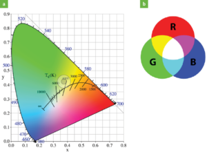

It is important to clarify the difference between light Color Temperature and Correlated Color Temperature (CCT). As stated previously, the concept of Color Temperature, properly defined and expressed, is based on an ideal black body radiator that emits a color based on its thermal temperature – in other words as a black body radiator heats up, the color it emits changes from red through yellow and white to blue. This definition lends itself well to the standard incandescent tungsten light bulb filament that works similarly – it emits a specific color temperature related to its resistive heating state.

However, LED and fluorescent lights do not emit light based on the thermal properties of a filament, and therefore the concept of Correlated Color Temperature (CCT) was defined and proffered. Based on human color perception, it quantifies the color expression accuracy of the light output. Thus, if a broadband light source (i.e. – white light) emits close to the black body Planckian locus, it can be modelled and expressed with its CCT. An excellent summary of light and color is located here:

https://www5.konicaminolta.eu/fileadmin/content/eu/Measuring_Instruments/4_Learning_Centre/L_D/The_language_of_Light/language_of_light.pdf

As seen in Fig. 14 (in the body above), we know that white LEDs are a comprised of a combination of a blue LED and a down-conversion phosphor coating. The resulting emission appears white to the human eye. Early attempts at creating white LED light showed considerable blue content in the spectrum, effectively creating the cold color temperature most often associated with surgical operating environments. As phosphor chemistry improved, multiple color temperature white LEDs were developed, each with a specific profile of blue and orange-red emission peaks (Fig. B7).

Additionally, we can take a closer look at the regions along the Planckian locus (see black line in Fig. B6) illustrating the color temperature “bins” an LED manufacturer specifies for one of their white LEDs (Fig. B8). LEDs are sorted after the manufacturing process into bins that are based on a range of properties including, forward voltage, light output power and color temperature.

In review, there are two important light specifications that assist in proper color reproduction:

Color Rendering Index (CRI)
Correlated Color Temperature (CCT)

For example, a common Quality Control inspection process in the automotive industry is differentiating / matching interior plastic panels. In fact, it is common for many Tier 1 or 2 automotive suppliers to produce specific grey color interior parts for multiple auto manufacturers, often each with subtly different “shades” and hues of gray. Suppliers will verify the gray scale of these panels to accurately match them with the corresponding auto manufacturer or model. Fig. B9 illustrates a generic example of the challenges involved with accurately reproducing the gray scale for identification / matching purposes, based on differing illumination CCT.

We can see here how differing color temperatures of white light can affect the image reproduction of flat gray (Fig. B9 – middle column under neutral light) and hence skew the differentiation, identification and matching between subtly differing gray to brown panels. With a substantial amount of preparation and testing, it is possible, however, to effectively calibrate a particular light’s CCT with a known part, thus creating a relative reference and correction factor. This approach usually involves testing all known part variations, and that can be difficult and time-consuming depending on the part source.

Additionally, for true color reproduction of non-gray objects and especially multiple color objects, specifying a particular CCT value lighting may not be sufficient. The color rendering index plays an important role here. CRI is best described as how well an object’s color is accurately reproduced in acquired images – compared to a standard. The higher the CRI, the better the color rendering accuracy. Most white LED lights have a CRI ranging from 70 to 95.

A typical request to machine vision lighting manufacturers regarding white LED color rendering accuracy, is whether a specific color temperature range or CRI value can be supplied. There is good news and bad news along these lines: The good news is LED manufacturers now offer a wide selection of both CCT and CRI; the bad news is oftentimes it is impossible to specify a very narrow range in CCT values. This is a limitation placed by the LED manufacturer, and is related to the LED manufacturing process itself. In any process of this type, there is a certain variation in both CCT and CRI over the  manufacturing run. LED yields are tested and “binned” according to certain ranges, and of course to optimize the salable yield, the manufacturer will opt to combine several adjacent sub-bins into one larger bin, meaning that one cannot typically purchase sub-bins. In practical terms, this implies that there is a range of values which manufacturers must use in the normal course of business. Fig. B8 shows an example of process binning and sub-binning around the ideal black body Planckian locus. In this instance, the combined sub-bins labelled as 1B + 1C + 1A + 1D, or 2B + 2C + 2A + 2D are only available at regular pricing and small volumes. A tighter binning, when even offered, usually requires premium pricing and large purchasing volumes.